Measures of Dispersion

Introduction to Measures of Dispersion

While measures of central tendency (like mean, median, and mode) provide a summary value representing the center of a dataset, they do not tell us how the data points are spread out around that center. This spread or variability is known as dispersion. In the context of pharmaceutical research and practice, understanding the dispersion of data is critical to assess consistency, reliability, and the degree of variation in parameters such as drug concentration, blood pressure, enzyme levels, tablet weight, or patient response to therapy.

Dispersion helps researchers understand how much variability exists in the dataset, whether the data values are tightly clustered around the mean (indicating consistency), or widely spread (suggesting unpredictability or inconsistencies in outcomes).

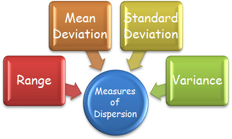
There are several methods of measuring dispersion, but three fundamental ones are: Range, Variance, and Standard deviation.

1. Range

The range is the simplest measure of dispersion. It is defined as the difference between the maximum and minimum values in a dataset:

Range = Maximum value − Minimum value

Explanation:

Though easy to compute, the range only considers two values in the dataset and ignores all the others. This makes it sensitive to outliers and not always reliable when making scientific decisions. However, it can give a quick preliminary idea of data variability.

Pharmaceutical Example:

Imagine a pharmaceutical analyst is measuring the dissolution time (in minutes) of 6 tablets of a new oral formulation:

Dissolution times: 32, 35, 33, 36, 34, 31

In this case:

• Maximum = 36 min
• Minimum = 31 min

Range = 36 – 31 = 5 minutes

Interpretation: The dissolution time of the tablets varies by 5 minutes. Depending on regulatory limits, this may or may not be acceptable. If tight uniformity is required, this range may indicate a need for formulation adjustment.

2. Standard Deviation (SD)

The standard deviation is the most widely used and reliable measure of dispersion. It quantifies how much each data point deviates from the mean. The more spread out the data is, the higher the standard deviation; the more consistent the data, the lower the standard deviation.

For a sample, standard deviation is calculated using:

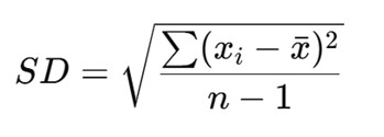
Where:

• xi = each individual value
• xˉbar = mean of the values
• n = number of observations

Pharmaceutical Example:

Suppose a batch of tablets is tested for active drug content (in mg), and the following five results are obtained:

Drug content: 98, 100, 102, 97, 103

Step 1: Calculate the Mean

Step 2: Calculate the Squared Deviations

(98−100)² = 4

(100−100)² = 0

(102−100)² = 4

(97−100)² = 9

(103−100)² = 9

Sum of Squared Deviations = 4 + 0 + 4 + 9 + 9 = 26

Step 3: Compute SD

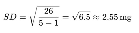
Interpretation: The standard deviation is 2.55 mg, indicating that most tablets deviate from the average drug content by around ±2.55 mg. If regulatory pharmacopeial standards allow ±5%, this would be acceptable for a 100 mg dosage. Otherwise, further refinement may be needed.

Importance in Pharmacy:

Standard deviation is critical in pharmaceutical quality control. It is used in:

• Tablet uniformity testing
• Bioequivalence studies
• Clinical trials (e.g., standard deviation of systolic blood pressure readings across treatment groups)
• Stability studies (e.g., variation in drug potency over time)

3. Variance

Variance is the square of the standard deviation and represents the average squared deviation from the mean. While it gives an idea about the spread of data, it is not in the same units as the original data, making it less interpretable on its own in pharmaceutical contexts.

Using the previous drug content example:

Interpretation: The variance is 6.5 mg², and the standard deviation is the square root of this (≈2.55 mg).

Although variance is mathematically essential, the standard deviation is preferred in practice due to its interpretability.

Pharmaceutical Problem: Application in Clinical Research

Let’s say a clinical trial evaluates the reduction in systolic blood pressure (SBP) after administering an antihypertensive drug. The reductions (in mmHg) for 6 patients are as follows:

Reductions: 12, 15, 13, 14, 10, 16

Step 1: Mean = (12 + 15 + 13 + 14 + 10 + 16) / 6 = 80 / 6 ≈ 13.33 mmHg

Step 2: Squared deviations:

• (12 – 13.33)² = 1.77
• (15 – 13.33)² = 2.78
• (13 – 13.33)² = 0.11
• (14 – 13.33)² = 0.44
• (10 – 13.33)² = 11.11
• (16 – 13.33)² = 7.11

Sum = 1.77 + 2.78 + 0.11 + 0.44 + 11.11 + 7.11 = 23.32

Step 3: SD = √(23.32 / 5) = √4.66 ≈ 2.16 mmHg

Conclusion: The average SBP reduction is about 13.33 mmHg, with a standard deviation of 2.16 mmHg. This means most patients experienced a reduction within 11.17–15.49 mmHg. The consistency of the drug’s effect can be judged based on this variability.

Conclusion

Measures of dispersion such as range, variance, and standard deviation provide valuable insights into the variability, consistency, and reliability of data in pharmaceutical sciences. While the range offers a quick but crude idea of spread, the standard deviation gives a more accurate and interpretable picture of how data points deviate from the mean.

In drug formulation, clinical trials, quality control, and bioequivalence studies, knowing how variable the outcomes are is as important as knowing the average. High dispersion might point to inconsistency in formulation, instability in active ingredients, or differences in patient response, all of which require scientific attention and adjustment.